Data Science in `vim`

Author

Seán Healy

Introduction

Code, email, blogs, notes: Almost everything I write, I now write in vim, so it’s become inconvenient when I have to use a program that doesn’t have a vim plugin. Muscle memory kicks in, and I find myself typing :w<CR> into textareas when posting online. As a sometimes-data-scientist, programmatic notebooks are an inevitable part of my workflow, and for a long time, I resigned myself to the fact that I would need to use a web-browser for this part of the work. Later I discovered VSCode’s Jupyter notebook plugin, which somewhat worked via a vim plugin, but not well enough. It was bug-laden in weird and unpredictable ways, sending me back to the browser. Then a few years passed, a few pieces of software got built, and I additionally found out about some pre-existing pieces. With these components, I’m now able to do all of my notebook work in vim, offline, while maintaining the presentation aspects of Jupyter notebooks.

This is one of my favourite things about working in Linux: different pieces of software can be easily combined in ways that the original authors never predicted. In my case, I have combined the following pieces of software to create a vim-based notebook workflow:

kitty: a terminal emulator that supports image rendering.
Neovim: a modern fork of vim, with support for multi-threading and Lua.
Molten: a Neovim plugin that allows you to run code blocks in a variety of languages and display the output graphics inline.
Quarto: a scientific and technical publishing system.

Component Parts

Kitty

Central to the programmatic notebook workflow is the notion of inline plots and images. The ability to display a plot right next to where its comprising data is loaded and manipulated: that sort of feature is beyond powerful. It reduces context switching and keeps the data scientist focused.

I suppose this is why Jupyter notebooks are used in the browser by default: browsers support images. Default vim, on the other hand, doesn’t support images. It’s a text editor. Terminals don’t support images, and vim also tendst to run inside a terminal. There are ways to sort-of display images and plots in a terminal: you can use ASCII-based plotting libraries, but the output is imprecise and archaic.

Kitty is a terminal emulator that supports full image rendering. It might even support GIFs, but I haven’t tried that yet. While working inside kitty, you can run kitty +kitten icat <image_path> to display an image inline. This is a crucial feature for a vim-based notebook workflow.

Installation (adjust for your distro):

emerge app-emulators/kitty

Something that you can only do in kitty:

kitty +kitten icat ~/headshot.jpg

It actually prints images to the terminal.

Neovim

It might be possible to use regular vim for notebooks, but I’ve been using the Neovim fork for years now. Both flavours are almost identical and they could even merge together someday. As far as I recall, Neovim handles multi-threading far better than vim, and includes support for Lua plugins and configurations. It’s also better maintained, so if you find a bug, it can be fixed far quicker.

Installation:

emerge app-editors/neovim

Molten

Molten is a Neovim plugin that allows you to run code blocks in a variety of languages and display the output inline. It supports a wide range of languages, including R, Python, Julia, and more. I primarily use R notebooks, because R is built for statistics, and it’s the default language for ggplot2, my go-to plotting library.

Before we can install Molten, we need the acquire a few more parts:

vim-plug: a plugin manager for vim and Neovim.
R: the best language for statistics and data visualization.
Jupyter: the ubiquitous programmatic notebook system.
ipykernel: a Python kernel for Jupyter notebooks.
IRKernel: an R kernel for Jupyter notebooks.

Installing Molten

It would nice if molten could simply be installed as a zero-dependency linux package, but it is new software, and things aren’t that easy yet. Instead, it needs to be configured, and different dependencies need to be pulled from a variety of package managing systems (Linux, R, Neovim).

We start with the linux packages:

# Install R, the Jupyter client, and Python kernel for Jupyter
emerge dev-lang/R dev-python/jupyter-client dev-python/ipykernel

Next, the R packages:

# Install the R kernel for Jupyter
R -e "install.packages('IRkernel'); IRkernel::installspec()"
# Install ggplot2
R -e "install.packages('ggplot2')"

vim-plug needs to be installed directly from GitHub:

curl -fLo "${XDG_DATA_HOME:-$HOME/.local/share}"/nvim/site/autoload/plug.vim \
    --create-dirs \
    https://raw.githubusercontent.com/junegunn/vim-plug/master/plug.vim

Installing Molten:

set nocompatible
filetype off

call plug#begin()

Plug '3rd/image.nvim'
Plug 'benlubas/molten-nvim'

call plug#end()

filetype plugin indent on " required

Configuring Molten:

let g:molten_auto_open_output = v:true
let g:molten_wrap_output = v:true
let g:molten_filetypes = {
\ 'python': v:true,
\ 'javascript': v:true,
\ 'r': v:true,
\ 'lua': v:true,
\ 'markdown': v:true,
\ }
let g:molten_image_provider = "image.nvim"    
let g:molten_virt_text_output = v:true

lua << EOF
require("image").setup({
    backend = "kitty",
    max_width = 800,
    max_height = 30,
    max_height_window_percentage = math.huge,
    max_width_window_percentage = math.huge,
    window_overlap_clear_enabled = true,
    window_overlap_clear_ft_ignore = { "cmp_menu", "cmp_docs", "" },
})
EOF

Jupyter Kernel

A Jupyter kernel is the component that executes the code in a Jupyter notebook. It is a headless process that runs in the background and communicates with the Jupyter client (the notebook interface) to execute code and return results.

Start the Jupyter kernel for R:

jupyter kernel --kernel=ir

Additionally, start the Jupyter kernel for handling Python code snippets:

jupyter kernel --kernel=python3

Quarto

Quarto is what I used to compile this blog post.

It’s a scientific and technical publishing system that allows me to create presentations, reports and websites. While parsing markdown files, quarto will actually execute the code snippets and include the output in the compiled HTML or PDF document. It does this independently of the Jupyter kernel, which is a slight annoyance, because that means I am running two separate programs for executing code snippets. It would be nice if the quarto vim plugin could display images inline, which would remove the need for Jupyter entirely, but it doesn’t support that, and this is why Jupyter and the Molten plugin remain useful for me.

Unless you’re on Ubuntu, you’ll need to install quarto from a tarball provided on its website:

Download the latest tarball from the quarto website, and install it like so:

tar -C /opt -xvzf quarto-*-linux-amd64.tar.gz
ln -s /opt/quarto-*/bin/quarto /usr/local/bin/quarto

There are two ways I use quarto, one for interactive writing, and another compilation process for the production-ready static HTML files. The first way happens like this:

quarto preview test_molten.qmd

The above command starts a local server based on the contents of the test_molten.qmd markdown file. An HTTP address will automitically open in your default web browser, and as you modify the test_molten.qmd file, the webpage will hot-reload your changes. Side note: .qmd is just a markdown file with some extra syntax highlighting for code blocks ( .qmd means ‘Quarto markdown’).

To generate HTML or PDF files, you can run the following command:

quarto render test_molten.qmd

Example Usage for OCR Analysis

First off, open a markdown file in vim or neovim (nvim):

nvim test_molten.qmd

Write something (anything) in markdown format:

# Introduction

Code, email, blogs, notes: Almost everything I write,
I now write in vim, …

As you save the changed file, the quarto preview server will hot-reload the changes, and you can see the output in the browser. I personally don’t love switching back and forth between browser and terminal, so I use the Molten plugin to run code snippets and display the output inline in the terminal. Then I intermittently check the browser to ensure my text reads well and that there are no syntax errors causing breakage during conversion to HTML.

Put your first code snippet in the markdown file: I’ll use a data file I have in my /tmp directory to show how this works.

library(ggplot2)
d = read.csv("/tmp/data2.tsv", sep="\t")
options(repr.plot.width=15, repr.plot.height=8)
head(d)

            method   oem0   oem1   oem2 combined
1     UPSIZED+NONE 0.9038 0.9712 0.9628   0.9822
2 UPSIZED+DENOISED 0.5572 0.6393 0.6303   0.6492
3  UPSIZED+NIBLACK 0.3035 0.7632 0.6401   0.7989
4  UPSIZED+SAUVOLA 0.8321 0.9469 0.9367   0.9597
5       UPSIZED+LI 0.9086 0.9439 0.9356   0.9705
6      UPSIZED+YEN 0.4685 0.8919 0.7836   0.8983

For those reading this in a browser, the above was achieved in markdown like so:

```{r}
library(ggplot2)
d = read.csv("/tmp/data2.tsv", sep="\t")
options(repr.plot.width=15, repr.plot.height=8)
head(d)
```

The format goes: three backticks, the language name within curly braces ({r} in this case). Then the block is closed with a further three backticks. Quarto will execute all code within blocks like these, unless the block is explicitly marked as non-executable. In this blog post, for example, wherever I am showcasing bash code, I do so with a special comment at the top:

```{bash}
#| eval: false
emerge app-emulators/kitty
```

This #| eval: false comment tells Quarto not to execute the code block, but simply render it with syntax highlighting if possible.

When the final line in a code block outputs text then it gets printed directly below the code. But what if the final line outputs a plot? Well, then it looks like this:

x = seq(0, 1, 0.1)
y = x
ggplot() +
        geom_point(aes(x=d$oem1, y=d$oem2)) +
        geom_line(aes(x=x, y=y), color="red") +
        xlab("OEM1") + ylab("OEM2") + theme_bw()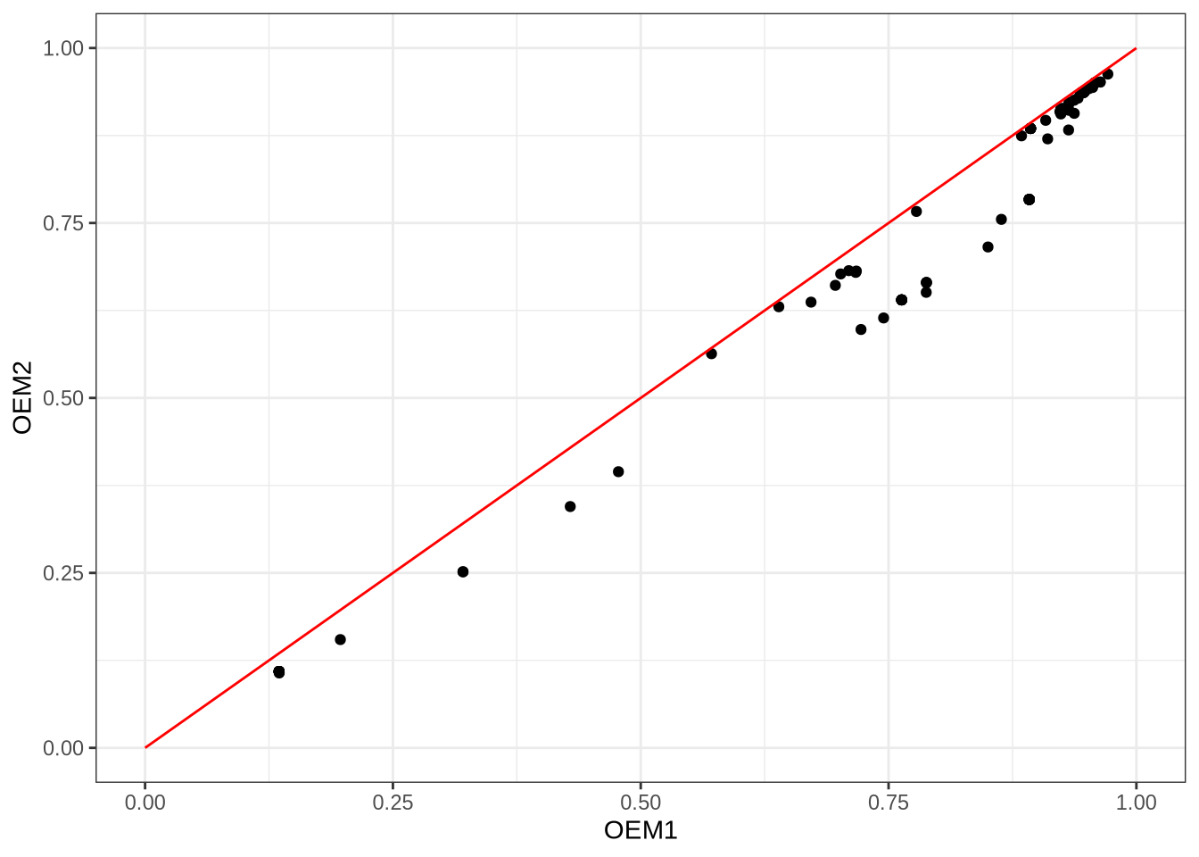

The above is just a piece of data visualisation I used to verify that it’s generally better to use the OEM1 option over the OEM2 option when doing OCR with Tesseract. OEM1 instructs Tesseract to use LSTM-based OCR, while OEM2 uses a combination of LSTM and legacy OCR. I was curious if the ensemble of legacy OCR and LSTM-based OCR would outperform the LSTM-based OCR alone, but it turns out that the inclusion of legacy OCR actually hurts performance. This is interesting given that I also found that legacy OCR can sometimes accurately recognise a word that LSTM-based OCR misses. The good does not outweigh the bad, it seems, and OEM2 fails to identify the specific moments when legacy OCR outshines LSTM-based OCR.

Back to the terminal, how would I display the above plot inline? Well, the Molten plugin allows me to do that, but it’s a very powerful plugin, so we need to further configure it first. Personally, I like the idea of using <tab> to evaluate code snippets, so I introduced the following lines into my Neovim configuration:

function NotebookSettings()
    MoltenInit
    nmap <TAB> ?^```{<CR>jV/^```$<CR>k:<C-u>MoltenEvaluateVisual<CR>
endfunction
autocmd BufNewFile,BufRead *.qmd call NotebookSettings()
autocmd BufNewFile,BufRead *.QMD call NotebookSettings()

What this does, basically: it checks if the file I’m working on is Quarto file (*.qmd or *.QMD), and if so, it runs a NotebookSettings function, which initialises Molten (MoltenInit) and then binds the <tab> key to a command that evaluates the code under the cursor. Let’s break that keybinding down:

nmap <TAB> ?^```{<CR>jV/^```$<CR>k:<C-u>MoltenEvaluateVisual<CR>
"aaa BBBBB ccccccccccDeFFFFFFFFFFgHiiiiiJJJJJJJJJJJJJJJJJJJJJJJJ

Label	Vimscript	Description
a	`nmap`	Create a keybinding in normal mode.
B	`<TAB>`	Bind to the tab key.
c	?^```{<CR>	Search backwards for the start of a code block.
D	`j`	Move the cursor down one line (to the first line of the code block).
e	`V`	Start visual line selection.
F	/^```$<CR>	Search forwards for the end of the code block.
g	`k`	Move the cursor up one line (to the last line of the code block).
H	`:`	Enter command mode.
i	`<C-u>`	Clear any existing command input (keybinding doesn’t work without this).
J	`MoltenEvaluateVisual<CR>`	Run the `MoltenEvaluateVisual` command, which evaluates the visually selected code block and displays the output inline.

With this keybinding in place, I can simply place my cursor on any line within a code block and press <tab> to evaluate the entire block and display the output inline. This is a game-changer for my workflow, as it allows me to stay focused in the terminal without needing to switch back and forth to the browser to see the results of my code.

Adding the Markdown YAML Front Matter

Markdown (and by extension, Quarto markdown) supports a feature called ‘YAML front matter’, which allows you to include metadata at the top of your markdown file. This metadata can be used to configure various aspects of how the markdown is rendered, such as the title, author, date. I used the following YAML front matter at the top of this file:

---
title: "Data Science in vim"
format:
  html:
    toc: true
    toc-depth: 3
    number-sections: false
    css: "test_molten_files/style.css"
  pdf:
    number-sections: false
execute: 
  cache: true
---

Fair warning: This YAML part doesn’t allow tab characters (two spaces for indentation). The cache: true line is a nice touch, as it tells Quarto to cache the results of code blocks, so that they don’t need to be re-executed every time you render the markdown file. I also like to include a custom CSS file for styling the HTML output (css: "test_molten_files/style.css"), and a PDF alternative for printers (pdf: number-sections: false).