tesseract <input.png> stdout txtOCR, Image Filters and Ensembles
OCR (Optical Character Recognition) is a technology that allows you to extract plaintext from image files: scanned paper documents, PDFs, or images captured by a digital camera. This is generally a first step in search indexing, custom language model pipelines. An app that allows you to photograph and digitize a receipt would rely on OCR. The more pixelated or blurry the image, the more difficult it is for OCR to work.
There are many tools available, ranging from expensive but near human-level solutions based on massive neural networks, or more efficient but less accurate solutions. There are also excellently performing solutions that are trapped inside GPT chat interfaces, where it becomes unreliable to expect the agent to respond with the intended format for each query. If you ask ChatGPT to process an image, annotate it in JSON format, 99% of the time it will respond with a JSON, but 1% of the time it will be natural language exposition or a combination of both. Using GPT at scale is also highly expensive, with each request for OCR costing around 3 cents per page. In a large scale OCR system, this would be prohibitive if not financially reckless given the possibility for system abuse.
I’m working on a business idea involving job matching and CV parsing, so naturally I needed an OCR pipeline to process CVs. I experimented with non-OCR solutions like pdftotext, but other CV building tools on the market don’t reliably output textual CVs. More often than not, the text within a CV is embedded in an image embedded right into the PDF. I would guess this is to make it more difficult for competition to process CVs, locking users into modifying their CV within the CV builder’s interface. Whatever the reason, I needed an OCR solution to ease user acquisition, and I started with the most ubiquitous OCR solution, Tesseract.
Tesseract is an open-source OCR engine that was developed by HP in the 1980s, and is now maintained by Google. Though it is known for its accuracy and speed, it fails with certain fonts and handwriting. Thankfully, CVs are formal documents, so handwriting and weird fonts tend not to be an issue.
There are a lot of moving parts with Tesseract. You can use it as a command line tool with default settings:
However, the program can do much more than this. It can also output bounding boxes around words, confidence scores, and alternate characters considered at each position in a word (confidence scores per character).
Legacy vs LSTM OCR Engines
Historically, Tesseract used some form of basic statistical analysis on a character-by-character basis to carry out its tasks. This is referred to in its documentation as the legacy engine. In 2018, Tesseract 4.0 was released, which introduced a new OCR engine based on LSTM (Long Short-Term Memory) neural networks. However, it is still possible to use the legacy engine, and in some cases it can outperform the LSTM engine. I’ve witnessed this myself on individual words, though it is rare. The LSTM engine is generally more accurate.
Usually an LSTM engine would be slower than more legacy statistical methods, but for reasons I haven’t explored, I’ve found that using the LSTM engine is actually faster than using the legacy engine.
The tesseract command line tool takes an --oem flag that allows you to specify which engine to use. The options are:
0: Legacy engine only.1: LSTM engine only.2: Legacy + LSTM engines
Based on what I’d expect from an ensemble method, I thought OEM option 2 would be the most accurate, but in my testing, it caused performance to degrade somewhat compared to using the LSTM engine alone. Whether this can be rectified, I haven’t yet determined, but I’m not throwing out the legacy engine just yet, as it does outperform the LSTM engine on certain words, and I reckon I can determine when exactly to use it.
First off, let’s get something straight. OEM1 (LSTM engine) is generally better than OEM0 (legacy engine):
library(ggplot2)
d = read.csv("/tmp/data2.tsv", sep="\t")
options(repr.plot.width=15, repr.plot.height=8)
x = seq(0, 1, 0.1)
y = x
ggplot() +
geom_point(aes(x=d$oem0, y=d$oem1)) +
geom_line(aes(x=x, y=y), color="red") +
xlab("OEM0") + ylab("OEM1") + theme_bw()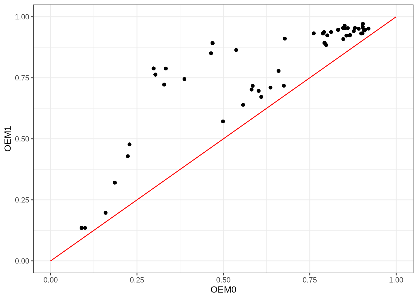
I took 100 CVs from online, generated synthetic data from them (PNGs), and used tesseract to process them with OEM0, OEM1, and OEM2. I then compared the recognised words against the ground truth text extracted from the PDFs with pdftotext. I used a variant of Damerau-Levenshtein distance that penalises character substitutions based on their visual similarity, so that for example, confusing an “o” for a “0” would be less bad than confusing an “o” for an “x”. There’s one point in the above plot for each CV page in my corpus. The x-axis is the OEM0 score, and the y-axis is the OEM1 score. All points lie above the red line (slope = 1), which means that OEM1 outperformed OEM0 on every single CV. However, there were still words that OEM0 recognised which OEM1 got wrong, and vice versa.
I was also curious about this OEM2 option, with the tesseract documentation vaguely describing it as a ‘combination of the legacy and LSTM OCR engines’:
ggplot() +
        geom_point(aes(x=d$oem1, y=d$oem2)) +
        geom_line(aes(x=x, y=y), color="red") +
        xlab("OEM1") + ylab("OEM2") + theme_bw()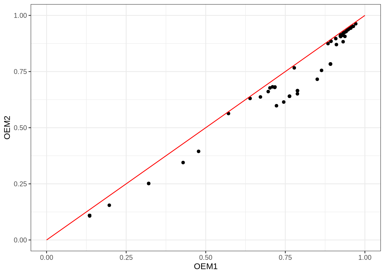
As seen above, things are not as clear-cut as OEM0 vs OEM1. However, it is apparent that combining LSTM with the legacy methods is ineffective, at least in whatever way Google does it. It could be the case that tesseract simply chooses the recognised word with the highest confidence score, not accounting for word rarity or prior knowledge of method performance. I am currently investigating if there is a better way to combine OEM0 and OEM1.
Pre-processing Images
After reading a few blogs that recommended pre-converting documents to high-contrast black and white in advance of tesseract, I decided to test this out. On my corpus of 100 CVs, I actually found that tesseract performed best on the original PNGs, and that pre-converting to black and white actually degraded performance. That said, for the words that were not correctly identified by tesseract on the original PNGs, some image filters did catch those words.
So should the original image alone be used, given it is the best performing on average? I don’t think so. At a pub quiz, you don’t want a team filled with the world’s best generalists. One excellent generalist is enough, and then a handful of specialists can give you that extra edge. In the same vein, why not run tesseract on both the original PNG and some variants that have been passed through filters?
What filters to use? There are many alternatives, and to complicate matters, each alternative has its own hyperparameters. Here is a non-exhaustive list of some image filters (thresholding methods) that I have experimented with:
- IsoData method
- Li’s method
- Local thresholding
- ImageMagick’s
-monochromefilter - Otsu’s method
- Sauvola’s method
- Triangle method
- Yen’s method
I also experimented with image sharpening filters. Among these methods, here are some that include hyperparameters that need to be tuned:
- Local thresholding has a
blocksizeparameter that determines the size of the local region used for thresholding. A smaller blocksize can capture finer details, but may also introduce more noise, while a larger blocksize can smooth out noise but may miss small features. It also has anoffsetparameter, but I don’t quite know what it does (my experiments found that it is best left at 0 for CVs). - Sauvola’s method has a
kparameter that controls the sensitivity to noise, and awindow_sizeparameter that determines the size of the local region used for thresholding. - Niblack’s method has similar parameters to Sauvola’s method.
- The
-monochromefilter in ImageMagick can be paired with astretchparameter used for stretching the contrast of the image. - Sharpening involves four parameters.
For each CV, I ran a genetic algorithm with a low population (I’ll fork out for a proper GPU rig one day, but in the meantime, N = 15 for my genetic algorithm is good enough). After a few evolutionary generations had passed without improved recognition accuracy, the algorithm would halt. This allowed me to find optimal hyperparameters for each filter and CV combination. Parameters would vary based on the CV being processed. Using these CV-optimal hyperparameters, I generated new images to feed into tesseract, and analysed the results.
What makes a good thresholding method for CVs?
‘Who’s the best odd-ball for your pub-quiz team?’ You know, the guy who won’t know the capital of Germany but will know the lead singer in a band called The The? This is what I think of when I consider how I might improve on state-of-the art OCR, while relying on a squad of image filters that tend to under-perform the default settings. First, let’s define what success looks like. A good odd-ball is someone or something that is good at the things few people are good at, and possibly bad at everything else. In the world of OCR, that means, we are not going to evaluate each thresholding method based on accuracy alone. We’re going to take those words that tesseract got wrong on the original PNGs, and see which thresholding methods get the largest proportion of those problem words right (I call this odd-ball accuracy). Later we can deal with the problem of determining when to trust the odd-ball over the consummate generalist. For now I just want to know who the best odd-balls are.
So I did a little experiment. I say little, because it was only a small amount of code. However, without a GPU, this actually ran on my computer for days. In that time, I realised there were a few other data points I should have collected, but the experiment had already started. Without going into too many details (email me if you’re interested in those), here were some of the results I found:
d = read.csv("/tmp/data6.tsv", sep="\t")
ggplot(d, aes(x=as.factor(rank), fill=method, y=count)) +
    geom_bar(stat="identity", position="dodge") +
    xlab("Rank") + ylab("Count") +
    scale_fill_brewer(name="Method", palette="Paired") + theme_bw()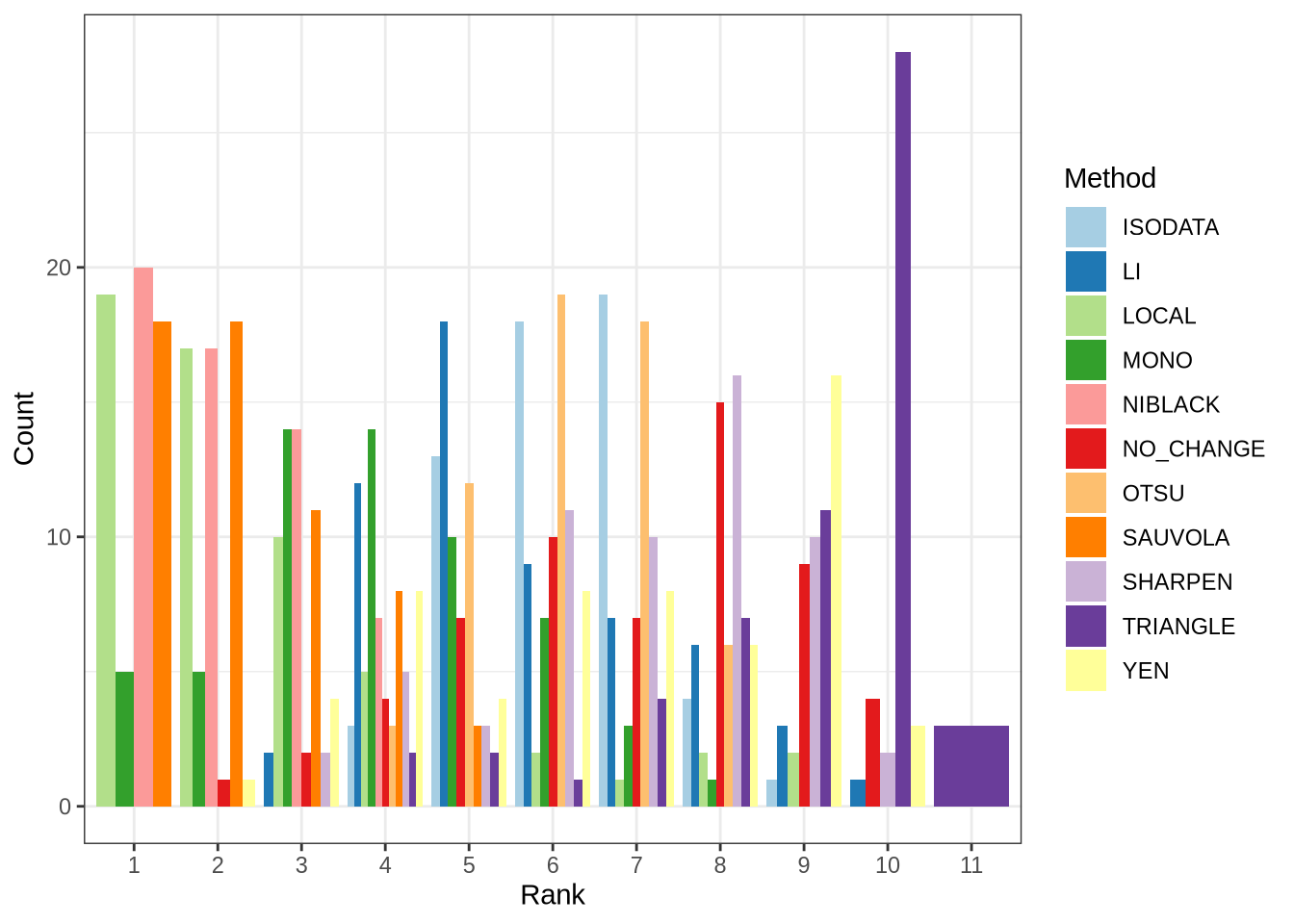
For each CV, I ranked methods based on their odd-ball accuracy score as discussed. The parameters used with each method were those found by the genetic algorithm. I found that the local, Sauvola, and Niblack methods were the best odd-balls, as these were most often the best ranked methods across CVs. The -monochrome filter worked best occasionally (dark green bar above), but not as well as those aforementioned methods. All other methods were comparatively poor, with the triangle method being the worst odd-ball.
What I learned from this experiment is that a combination of the original PNG, and variant images generated with the local, Sauvola, and Niblack methods, is likely to yield the best results when fed into tesseract. This assumes that we can find a way to determine when to trust the odd-ball over the generalist.
Continuing with the pub quiz analogy, if two team mates are now chosen: original PNG (the generalist), and the Niblack thresholding method (first odd-ball), the next question is, who will be the third team mate? The earlier definition of success can be amended based on the combined performance of the generalist and first odd-ball. This would produce a set of words that are a subset of the earlier discussed problem words. Call these very troublesome words. The next odd-ball can be evaluated on its ability to correctly identify these very troublesome words. Repeat this until the team is filled. This greedy approach to team selection is not guaranteed to produce the optimal team, but it is a simple heuristic that can be implemented without too much computational overhead.
The problem of how best to combine results from each method is something I’ll investigate next.